Context

The Carr-Madan decomposition is used in quant finance to break any payoff into a (continuous) combination of calls and puts, plus a forward. Namely, for any twice differentiable function:

\boxed{ f(x) = f(y) + f'(y)(x-y) + \int_{-\infty}^y f''(z) (z-x)^+ dz + \int_{y}^\infty f''(z) (x-z)^+ dz }

where $(x)^+ \equiv \max(0, x)$ is the positive part function.

This result translates what quants intuitively know: for a derivative product with any given payoff, we can approximate it from calls and puts (plus a forward).

More specifically, we will approximate the integrals as Riemann sums: let $L >0$ be some sufficiently large value. Then

\begin{align*} f(x) &\approx f(y) + f'(y)(x-y) \\ &+ \sum_{i=0}^{N} f''(z_i)(z_i-x)^+\quad \text{where}\quad z_i \equiv -L + i \Delta z, \quad \Delta z = \frac{y+L}{N}\\ &+ \sum_{j=0}^{N} f''(z_j)(x-z_j)^+\quad \text{where}\quad z_j \equiv y + j \Delta z, \quad \Delta z = \frac{L-y}{N}.\\ \end{align*}

We will then have a total of $N+1$ calls and $N+1$ puts.

import numpy as np
from numba import jit
import matplotlib.pyplot as plt

# original function
def f(x):
    return np.cos(x)

@jit(nopython=True)
def series_expansion(x, y, N=100, L=10):
    
    def f(x):
        return np.cos(x)

    def df(x):
        return -np.sin(x)

    def ddf(x):
        return - f(x)
    
    summand = f(y) + df(y)*(x-y)
    
    dz = (y+L)/N
    for i in range(1,N):
        z = -L + i*dz
        summand += ddf(z)*np.maximum(z-x, 0)*dz
        
    dz = (L-y)/N
    for i in range(1,N):
        z = y + i*dz
        summand += ddf(z)*np.maximum(x-z, 0)*dz
        
    return summand

Using 100 terms:

x_range = np.arange(0, 10, 0.01)
carr_madan = [series_expansion(x, 1, N=100, L=50) for x in x_range]

plt.plot(x_range, carr_madan, label='Carr-Madan approx')
plt.plot(x_range, f(x_range), label='True function')
plt.legend()
plt.show()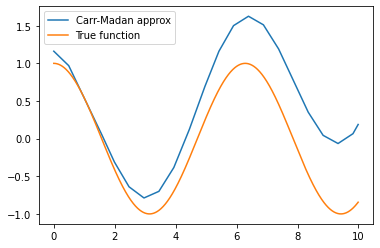

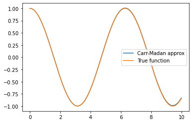
png

Increasing to 10,000 terms: the approximation gets much better.

x_range = np.arange(0, 10, 0.01)
carr_madan = [series_expansion(x, 1, N=10000, L=50) for x in x_range]

plt.plot(x_range, carr_madan, label='Carr-Madan approx')
plt.plot(x_range, f(x_range), label='True function')
plt.legend()
plt.show()

png

The Carr-Madan decomposition of arbitrary payoff functions

Context

You may also enjoy: