Introduction
This article introduces PDE-constrained optimization, a discipline with deep applications in engineering design. After all, any physical law is represented by a PDE, and engineering cares a lot about finding optimal designs — lower costs, higher safety, better performance, you name it.
We will navigate from good old Lagrange multipliers in to infinite-dimensional functional derivatives. Buckle up.
In first-year calculus, we learn how to optimize a function, i.e. to find the maximum or minimum of a function . Namely, we need to “differentiate and equal to zero”:
A bit later, we learn that we may also add constraints to this optimization business: it may happen that cannot take all possible values, but only those implicitly defined by . We then introduce the notion of a Lagrange multiplier, usually written as , and consider the modified function
and our goal becomes to now find the values such that
There are various ways to generalize this framework, e.g. considering inequality constraints instead of equalities.
In applications, especially when dealing with physical systems, this framework may be too simple to capture the complexity of the real world. We need to generalize it.
A motivating example
Instead of starting with the abstract framework, let me first motivate it with an example.
An aerospace engineer is working a project to transport various types of gases to Mars. She is given a task of designing a container in the shape of a hollow aluminum spherical shell with a radius of 2 meters, that must withstand an internal pressure of 250 kPa while being transported in outer space (so the outer pressure is 0). This is the same pressure inside a can of soda in room temperature.

Like this, but larger. Picture from the internet.
There are two catches here:
- Any solid, under pressure, will deform. Our project requirements specify that the maximum allowed deformation of the container is 3 mm.
- Transporting massive objects in space is very expensive. Therefore, we want the mass of this container to be as small as possible.
What should our engineer do?
First, she parameterizes the problem. The geometry is fully determined by the radius of the sphere, , and its thickness , with the former being fixed at meters. The design variable, analogous to the abstract variable in the previous section, is just the thickness .
How to map this variable to the total mass and maximum deformation of the shell? For the mass, the engineer know hows to proceed: since we are talking about a thin spherical shell (i.e. ), its volume is just the surface area of the sphere multiplied by the thickness, i.e.
and hence the total mass is just this volume multiplied by the density of aluminum:
Great - she knows what she wants to minimize as a function of . This is the equivalent of our optimization function discussed above.
But now she encounters an issue: how to write down the function describing the constraints to her problem? The constraints are the laws of physics themselves! In this particular case, she needs to solve the partial differential equation (PDE) for linear elasticity considering the boundary condition of 250 kPa pressure inside and zero outside.
The solution to this equation is a displacement field describing how a point inside our massive body gets displaced to a new point . In this way, the displacement field describes how the body deforms under pressure. If she was given it, she could impose the requirement
Notice how the flow of information goes, starting from the parameters describing the geometry:
PDE-constrained optimization is a complex task that will be the focus of our discussion today.
Luckily for our engineer, she realizes that, in this case, spherical symmetry simplifies the problem significantly - browsing through her books, she finds an exact solution for the displacement of a spherical shell under internal pressure :
where are parameters (Young’s modulus and Poisson ratio) describing the stiffness of aluminum (this equation appears in Landau & Lifschitz Volume 7, Paragraph 7, Problem 2).
How lucky she is! She can finally write down her problem as follows: considering that, for aluminum,
- Density:
- Young’s modulus:
- Poisson ratio:
and that the pressure for this problem, the optimization becomes
This is now easy to solve: since the function to minimize is linear, we want to pick the smallest possible value of satisfying the constraint. Since
we conclude that the optimal value for is 1.59 millimeters, corresponding to a total mass of 218 kilograms.
Our engineer sighs in relief that the formula for the displacement of a spherical shell was available analytically. She wonders what she would have done if it wasn’t…
The general framework
Leaving the example, we now introduce the theoretical framework.
Our ingredients are fourfold:
Ingredient 1: a function which is a solution to a differential equation and its initial / boundary conditions. Both and its argument can be almost anything: vectors, scalars or tensors, real or complex.
Ingredient 2: we further assume that something - maybe the geometrical domain over which is defined, or its boundary conditions - can be parameterized with a set of parameters , considered here as a finite vector. In the previous example was a single vector with the thickness of the shell.
Then, will be indirectly a function of as well as of its variable . We may write this as or when we want to explicitly communicate this dependence.
Ingredient 3: We are also given physical and/or design constraints that we want our solution to satisfy.
These can be human-chosen functions, but also the laws of physics themselves - in the previous example, we had both the upper limit on desired deformation of our shell but also the linear elastic equations. In all generality, write them as . As functions of , these will inherit the dependence on .
Ingredient 4: finally, we are given a scalar functional, called a loss function or objective function, and often written as , that takes in and returns a real number. is what we will want to optimize for.
A functional is just a function of a function. In physics, to make the difference between a regular function and a functional explicit, we use square brackets for their arguments instead of parenthesis. Hence, is a functional taking in a function, and returning e.g. a number (or maybe another function)
As a function of , is indirectly a function of ; in some cases, we may also explicitly pass as an argument to , as was the case of the previous example in which was the mass of the shell - it did not depend on , but depended on the thickness directly. Below, we will write
depending on the context.
Examples of this framework are:
Designing a heat sink:
- is the temperature field over the heat sink, which solves the steady heat equation
- specifies design parameters, such as fin spacing, height or thickness
- A design constraint may be that maximum temperature at specific points does not exceed some threshold
- may be the heat flux integrated over the base of the heat sink, as a measure of its efficiency.
Designing an airfoil for a plane
- is actually a tuple describing the air velocity and pressure over the airfoil. The equation is the Navier-Stokes equation of fluid mechanics
- can be any set of parameters describing the shape of the airfoil
- Design constraints may include target lift-to-drag ratios
- may be the drag force, which we want to minimize.
As we can see, this framework is pretty general. Adjoint methods are one way of tackling this very broad family of problems.
The need for derivatives
In the literature for adjoint methods often focuses strictly on a slightly different problem:
That is, how can we precisely calculate the sensitivity of the objective with respect to the parameters ?
Of course, computing derivatives and optimizing are related tasks - we discussed this in the beginning of this section. Many optimization methods, such as the famous gradient descent method and its variants, directly rely on computing gradients. Even for problems which are not strictly optimization tasks, such as solving a non-linear equation, can benefit from derivative information, as is the case with the Newton-Raphson method.
Therefore, knowing how to compute the derivative of our objective function is an important task on its own, and one that can be used directly in optimization. Therefore, this will be our focus from now on.
Aren’t finite differences enough?
A naive (but nonetheless useful and still very used in practice) way to compute the sensitivity of with respect to is to slightly perturb and recompute , approximating the derivatives via finite differences.
Namely, suppose one has access to a function that, given a vector , yields the solution function . Then, we can approximate the -th component of the vector , at a particular value , as
i.e. as the finite difference approximation along axis with unit vector (other approximation methods, such as central differences, can also be used).
This can get expensive very quickly: on top of calculating , this involves calls to if takes values in . Calls to differential equation solvers (both ODE and PDE) are almost always expensive.
Therefore, especially when dealing with many parameters, there are better ways. We discuss them now.
Motivating the adjoint
For concreteness, assume for now that takes values in and takes values in . Then, schematically,
Both the LHS and the first term in the RHS are (row) vectors. The last, product, term, is the matrix product of a (row) vector and a matrix, yielding the correct dimensions.
The first term on the RHS is something that often will not depend on the solution of a PDE (for example, how mass depends on the geometrical parameters). It can be computed in a variety of ways, from automatic differentiation to finite differences.
Similarly, the term can often be calculated explicitly since is a human-chosen metric. Therefore, the complexity lies in calculating : how the solution to the PDE depends on its parameters.
Let us assume that a set of constraint equations
are given, with taking values in . If these equations hold identically, then in particular their total derivative with respect to must be zero as well:
Plugging back into the expression for gives
Let us give a name to the term : call it the adjoint
which can be seen to be the solution of a linear system of equations:
(again, check for matrix dimension consistency: is a matrix, and the RHS is a column vector, so must be a column vector).
Then the total derivative w.r.t. parameters can be found as
This is a very interesting result. It shows that, regardless of how is obtained (for example, as the solution to a complicated boundary value problem), once we have it, we can use it to compute the adjoint via its linear system; the solution can the be plugged into the expression above to immediately obtain sensitivity. This did not require many calls to the DifferentialEquationSolver!
Lagrange multipliers and adjoints
An alternative derivation of the adjoint equation utilizes the method of Lagrange multipliers. This approach provides additional insight by embedding the constraint directly into the functional, allowing us to treat the solution process and optimization problem simultaneously.
We start by defining an augmented functional — the Lagrangian — that includes the constraint :
where is a vector of Lagrange multipliers, also referred to as the adjoint variables, and takes values in .
For the total derivative to be consistent with the constraint , we require stationarity of with respect to all variables. This means that the partial derivatives of with respect to , , and must vanish:
- Stationarity with respect to enforces the constraint:
- Stationarity with respect to yields the adjoint equation:
This is the same linear system for as derived earlier.
- Stationarity with respect to yields:
Assume we have found , , satisfying the required equations. Then the condition is satisfied; on this set of parameters, the Lagrangian just equals itself, and
which is given by the equation above. Hence, we find the same expression for sensitivity as before!
Continuous adjoints
The Introduction motivated the construction of adjoints as auxiliary variables for calculating sensitivities of objective functions with respect to their parameters.
For this, we assumed all quantities were finite; in particular, that the constraints could be represented by a vector equation with components. was then also a vector in .
However, in the general case, we will be dealing with infinite-dimensional spaces; solutions of PDEs commonly live in Banach spaces. Therefore, we must generalize the discussion above to infinite dimensions.
As a spoiler, if you are only interested in finite element methods (FEM), then you can freely skip this section. FEM brings functions from infinite-dimensional spaces to finite-dimensional representations, and so the machinery of the previous section applies nicely - in particular, the laws of physics become a finite system of equations.
Gateaux derivatives
Writing a section with the right balance between mathematical rigor and intuition is always challenging. Since my main focus here is giving you the tools for computing things, I will provide a mostly operational definition of the necessary mathematical entities.
Recall that a functional is a function taking in another function, say , and returning a number. We may write in the same way we write for a function taking in an argument .
The Gateaux differential or Gateaux derivative of a functional is a linear operator defined by its action on any function as
A few comments are in order. First, notice that does not exist by itself; it is only defined when applied to another function .
The is a pairing notation that is reminiscent of an inner product, but this is just notation. It is made to evoke the usual directional derivative in Euclidean space, namely . There are alternative notations; see below.
The possible domain of functions is the same of . More precisely, if are Banach spaces and is an open set, let us assume . Then, is defined for any and .
Secondly, notice that we could equivalently write the RHS of this definition as
this is indeed how many books define this derivative. I find the notation we used more useful for most applications, but both are equivalent.
A word on notation
The notation above is not unique. It is closest to that of reference [3] with the square brackets coming from the convention in physics for functionals.
The following are other equivalent notations observed in the literature:
Physics tests further define the so-called functional derivative as the integral kernel of the Gateaux derivative, i.e. a Gateaux derivative “density”. More precisely, for a functional given by an integral
the functional derivative is the quantity defined via
where we have written instead of .
Physicists’ notation is slightly more compact and generalizes easily for more than one functional. For example, if then its total Gateaux derivative is just
Imposing, for instance, that would require both integrands to be zero for any variations .
Example calculation
We now provide an example to make the calculation of Gateaux derivatives more concrete. Let . Consider functions which are square-integrable over , taking real values. For some smooth function , define
Let us calculate its Gateaux derivative:
which shows that the Gateaux derivative is the linear functional given by
Exercise: generalizing the case above for , show that
Exercise: in the case above, specializing to test functions which vanish on the boundary , show that requiring for all implies the Euler-Lagrange equation:
Optimization for the heat equation
Our working example will be that of the heat equation. We do this to avoid excess abstraction in the theory, while providing a concrete application which you can use as inspiration for other problems.
Weak form
Weak formulation of the heat equation in with mixed Neumann and Dirichlet boundary conditions: the equation is, in its full glory,
(with ). Here,
- denotes temperature, in whatever chosen units (e.g. Kelvin)
- is the thermal conductivity, in units of power per unit length, per unit temperature
- is some internal energy source density, in units of power per unit volume
- is some prescribed flux, in units of power per unit length.
By multiplying by a test function and integrating by parts, we are able to rewrite the problem in its weak (continuous Galerkin) form as: find such that
where
and where we have defined the following subspace of
Setting up the Lagrangian
Let us assume that we want to minimize the following functional, sometimes called heat transport potential capacity (see reference [2]):
The intuition behind this quantity is that it measures how well temperature flows around the body.
Great, we have an objective to optimize for. Now, what are our parameters ?
In this functional framework we are in, we want to be able to ask questions such as “how would my objective function change if I perturbed this function?”. A common function to choose in the heat scenario is itself — the thermal conductivity. This is particularly true in topology optimization scenarios in which we want to let become zero in some regions, effectively introducing holes in the medium.
Therefore, let us work with this assumption: our parameter in this case will be the thermal conductivity itself. This is a good example since it appears both in our objective and in our constraint equations.
We need only add a Lagrange multiplier and the associated constraint to this functional, and we will have in our hands a Lagrangian that we can optimize. Gateaux derivatives are the tool of choice for optimization when we are dealing with infinite-dimensional functionals, analogous to how the regular derivative was our tool for finite-dimensional optimization.
I assert that
is the Lagrangian we want, with the test function that appears in the weak formulation being our continuous Lagrange multiplier.
It does not explicitly appear in the neat form Lagrange multiplier times constraint that we are familiar with, but this is purely aesthetical: remember that the weak form was obtained by multiplying the strong form by and integrating. That is,
where here is the inner product
Therefore, what we have above is a sum (integral) of the Lagrange multiplier times the constraint at every point .
Calculating derivatives
For completeness, I repeat here what our Lagrangian is:
Things are about to get a bit mechanical since we are entering the domain of “sit down and calculate”, but we can foresee what is going to happen. Remember from the first chapter that, for a simple Lagrangian (renaming to to match current notation)
we had that:
- Stationarity w.r.t. gave us the constraint equation
- Stationarity w.r.t gave us the adjoint equation, i.e. that solved by ;
- Stationarity w.r.t. gave us the desired equation for the sensitivity of with respect to the parameters
The same thing will happen now. We will first be very explicit with the Gateaux derivatives, to help you get used to the machinery.
If we were using physicists’ notation as discussed in the previous section, we could just take with an understanding that this would generate 3 sets of terms: those proportional to , and , respectively, all which would have to be zero independently.
Stationarity with respect to the Lagrange multiplier
Only terms containing and its derivatives are non-zero, so we can ignore (I). Starting with (II):
You may realize that, whenever the functional is linear in and its derivatives, the Gateaux derivative formally just replaces with . For example, (III) yields
In fact, we can find ourselves a nice general result beyond the heat equation here. Recall that our Lagrangian is, on a high level,
since the term does not count for the derivative with respect to , and since both and are linear forms with respect to , we immediately conclude that
But is literally the weak form of our problem. Therefore, we have just retrieved the constraint equation, as expected.
Stationarity with respect to the solution
We now go back to the derivative with respect to . The derivative of the objective function (term (I)) is:
Notice the test function is now ; for every stationarity condition, we use a new test function. This is more easily seen in physicists’ notation, in which would be .
For term (II), we notice it is a linear function of and, from the discussion in the previous section, we know that
Finally, terms (III) and (IV) are not functions of , so they can be ignored. Putting everything together, we find that
Notice that this can be written as
which, in turn, implies the surprising result
i.e., for the particular case of the objective function given by the heat potential capacity, the adjoint is equal to up to a sign.
Can you see why this would not be the case if we had chosen any other ?
An addendum: the strong form of the adjoint problem
Although we found ourselves a nice result in this case, it would not be like this had we chosen other objective functions.
Let us pretend we didn’t see that, and instead do something different: starting from the weak-form adjoint equation,
let us show that we can actually reverse-engineer the strong form PDE for the adjoint .
The trick is to integrate by parts so that appears without any derivatives. This procedure will result in bulk and boundary integrals which must all independently vanish. Let us see how.
Writing
and integrating by parts, we get
We can simplify this expression in several ways:
- The integral vanishes since , i.e. vanishes over
- On ,
- In , the strong form of the primal problem is
Hence, the equation becomes
For both integrals to vanish, we obtain the differential equation
and boundary conditions
Notice that formally replacing yields exactly the strong form problem for , which reinforces that this is the solution for the adjoint in this formulation.
Going back to derivatives
Stationarity with respect to parameters
Finally, we calculate the derivative with respect to , or in this particular example. Only terms (I) and (II) depend on , which appears linearly in both, so we immediately find
But we know that, for our problem, we have a nice analytical result: , which we can substitute to obtain
showing that, for an everywhere non-negative change to (specified via ), our objective function will become smaller.
Does this make sense, physically? Assume a very simple case, that of a solid beam-like structure. We set in one end (say, at ) and specify the flux at the other end (say ).
Since the problem is 1D, the heat equation is just , with solution matching the boundary conditions. The higher is, the less of a temperature drop between and we observe - good conductors spread temperature across them more effectively.
The heat potential capacity can be calculated analytically to be
Indeed, if we let increase, decreases, in accordance to what we just found:
Joining everything
We are done:
-
We pick an objective function , here being
-
We solve the primal problem to find satisfying
where
and the relevant space is
-
Then, we solve the adjoint problem, which depends on and the solution of the primal problem. In this case
-
With these two in hand, we can compute the sensitivity of our loss with respect to the thermal conductivity along any “direction” , interpreted as a perturbation to via
Discrete adjoints and FEM
In practice, despite the continuous formalism’s elegance, for computational purposes we need to restrict ourselves to finite dimensions.
Lightning review of FEM
This is the whole deal with the Finite Element Method (FEM): starting from the continuous formulation on an infinite-dimensional vector space , namely
the finite element method invites us to find a finite subspace , spanned by a basis , such that we can write
If the form is bilinear and is linear, we can plug these expressions in and write
For this to hold for any ‘s, it must be true that (calling and ):
or, in matrix form
with being a matrix whose component is , and being column vectors.
Therefore, making use of a FEM-like basis expansion, we are able to reduce our infinite-dimensional, continuous approach into a matrix equation.
Optimization problem revisited
This program of converting our quantities into matrix objects can be expanded to the objective function as well. For instance, consider our objective
In FEM, we discretize the domain into a mesh of, say, tetrahedra - the elements. The basis functions are then constructed so that they are localized, each being non-zero only over a few such elements.
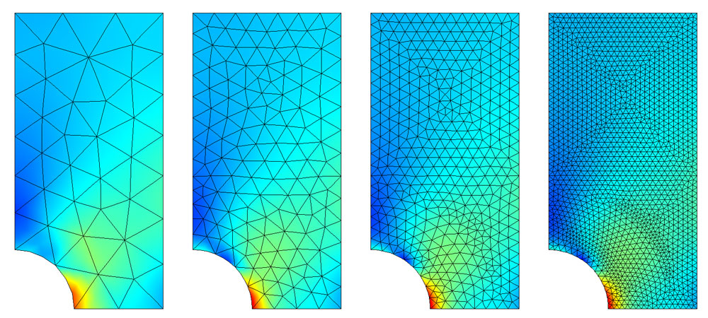 Example of a 2D domain being meshed to increasingly finer resolutions. From COMSOL documentation
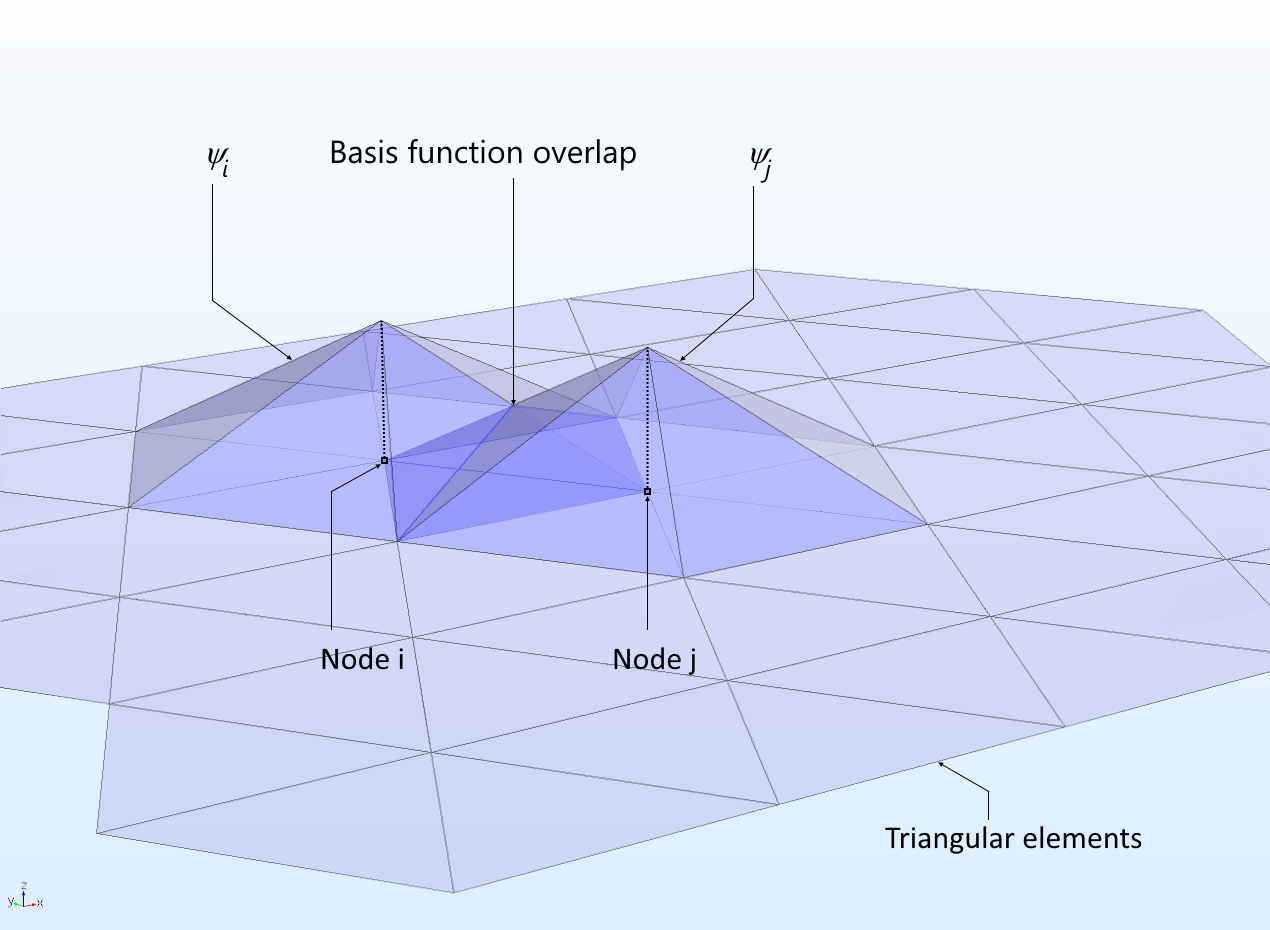 Example of two basis functions and their overlap. Notice that, outside the highlighted areas, the basis functions are identically zero. From COMSOL documentation
Assume we are given such a mesh, consisting of tetrahedral elements . We will make the assumption that can be approximated well enough element-wise, i.e. is a constant per element.
This greatly simplifies the integral. Since the gradient can be written as
we can approximate the integral as an element-wise sum:
Defining the stiffness matrix
although initially a operation, it is actually much faster to calculate since each has a small support, making a sparse matrix. We finally find
where the matrices and are defined naturally.
Hence, our full optimization problem becomes
This is a properly-defined quadratic optimization problem, which can be naturally tackled via Lagrange multipliers as explained in the first chapter.
The FEM heat equation
Since we did so much work for the heat equation in the continuous case, let us see that we get essentially the same equations for the discretized case.
Write our Lagrangian as
where we should explicitly calculate the relevant matrices. We defined
Using an element-wise constant , this boils down to
Similarly, we defined
which can also be converted to an element-wise sum over 3D and 2D elements if we choose to represent and as element-wise constant.
Finally, we recall that we defined
Oh, but wait — this is exactly the expression for that we found before. Again, the fact that we chose a very specific has helped us, since it gives the nice result
It is trivial to see that taking the derivative yields the constraint equation (notice that is a row vector, since is defined as a column vector). Let us then compute the derivative with respect to . Everything is more easily done in index notation, since
Then the -th component of the derivative with respect to is easily seen to be
where we have replaced with . This can be shifted back to matrix notation:
which, when set to zero, gives
as before!
Finally, we can take the derivative with respect to - or, more precisely, against the vector whose number of components is the number of mesh elements.
We have
Using that yields
Now,
and the matrix product becomes
Therefore, we conclude that is a -dimensional vector (one component per mesh element) whose components are the quantities
for each . Convince yourself that this is the discrete analog of the Gateaux derivative
obtained in the continuous case.
Future to-dos
This is getting pretty long as it is, so we will call it a day for now. After motivating the importance of PDE-constrained optimization, we started with Lagrange multipliers in finite dimensions; went up a layer of complexity to study adjoints in the continuous case; and then came back to finite dimensions with the help of FEM. As we saw, the constructions are equivalent in the sense that, when projected to finite dimensions, they yield the same equations.
As next steps:
- Add FEniCSx implementation of an adjoint
- Add more examples and exercises, especially with other objective functions
References
-
Bradley, Andrew M. “PDE-Constrained Optimization and the Adjoint Method.” Published July 7, 2024. Originally November 16, 2010. https://cs.stanford.edu/~ambrad/adjoint_tutorial.pdf.
-
Guo, Zengyuan, Cheng Xinguang, and Xia Zaizhong. “Least Dissipation Principle of Heat Transport Potential Capacity and Its Application in Heat Conduction Optimization.” Chinese Science Bulletin, vol. 48, no. 4, 2003, pp. 406-410.
-
Allaire, Grégoire, François Jouve, and Anca-Maria Toader. “Structural Optimization Using Sensitivity Analysis and a Level-Set Method.” Journal of Computational Physics, vol. 194, no. 1, 2004, pp. 363–93. https://doi.org/10.1016/j.jcp.2003.09.032.